Speculative Speculative Decoding Explained

If you have worked with large language models in production, you have probably faced this problem:

Models are powerful, but they are slow.

Even with good GPUs, generating responses one token at a time adds latency. For real-world applications like chat systems, copilots, or voice assistants, this delay is noticeable and often unacceptable.

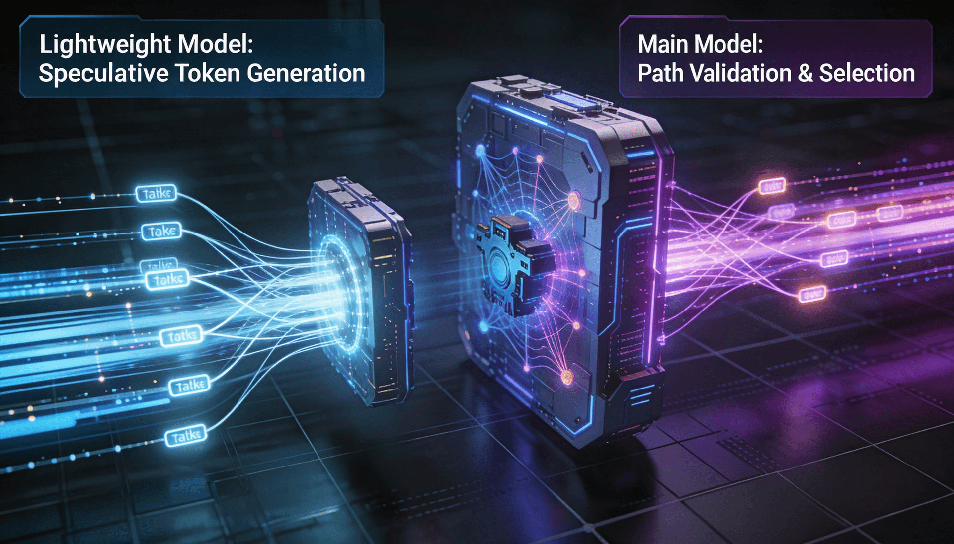
Several techniques have been proposed to speed up inference. One of the most effective is speculative decoding, which uses a smaller model to guess the next few tokens and a larger model to verify them in one pass.

But speculative decoding still has a problem. It is sequential. The draft model has to wait for the target model to finish verifying before it can start guessing the next batch of tokens.

This is where a new approach comes in:

Speculative Speculative Decoding (SSD), Instead of just improving the draft model, SSD parallelizes the draft and verification steps entirely. The draft model pre-computes possible futures while the target model is still verifying, so the next round is ready the moment it's needed.

In this blog, we will explore what SSD is, why it matters for modern AI systems, how it works internally, what I implemented in my proof of concept, and the kind of real-world performance improvements it can deliver for LLM inference.

What is Speculative Speculative Decoding?

Speculative Speculative Decoding (SSD) is an inference technique designed to reduce latency in large language model generation. Instead of generating tokens one by one, SSD predicts multiple future possibilities in parallel, so the next steps are already prepared before the current verification finishes.

It builds on speculative decoding but adds parallelism inside the decoding loop. In standard speculative decoding, the draft model sits idle while the target model verifies. In SSD, the draft model runs on separate hardware and starts preparing the next round of speculations while the verification is still in progress.

The optimized version of SSD is called Saguaro. According to the paper, it achieves up to 2x speedup over speculative decoding and up to 5x speedup over standard autoregressive decoding.

SSD is lossless. The output is identical to what the target model would produce on its own. There is no trade-off between speed and accuracy.

What Problem Does SSD Solve?

The first problem starts with how LLMs normally generate text.

1. Traditional Autoregressive Decoding

In standard LLM inference, tokens are generated one at a time:

• Generate one token
• Feed it back into the model
• Generate the next token
• Repeat

This process is called autoregressive decoding, and it is inherently sequential. Every new token depends on the one before it, which means the model cannot fully parallelize generation.

That creates several problems:

• Responses become slower as output length increases
• GPUs stay underutilized during generation
• Latency becomes noticeable in real-time applications like chatbots, copilots, and voice agents

Even extremely powerful GPUs cannot avoid this bottleneck because the model still has to wait for each token before moving to the next one.

2. Speculative Decoding (First Improvement)

Speculative decoding improved this:

•       A small draft model generates several candidate tokens quickly

•       A large target model checks them all in one forward pass

This lets us generate multiple tokens per step instead of one.

But there is still a bottleneck:

•       Draft → Verify → Draft → Verify

•       The draft model waits during verification. The target model waits during drafting.

SSD (Next Step)

SSD removes this waiting by overlapping drafting and verification.

The draft model runs on separate hardware. While the target is verifying the current round, the draft model predicts what the verification result will be and prepares the next round of speculations ahead of time.

These are stored in a speculation cache. If the prediction is correct (cache hit), the next speculation is returned instantly with zero wait. If the prediction is wrong (cache miss), it falls back to standard speculative decoding.

LLM Decoding Methods Compared

Here is a side-by-side comparison of autoregressive decoding, speculative decoding, and SSD across speed, execution flow, and hardware usage.

How SSD Parallelizes Decoding

SSD is based on a simple concept, similar to speculative execution in CPUs. In CPUs, the processor runs both branches of an if-statement before knowing which one is needed, then throws away the wrong one. SSD applies the same idea to language model decoding.

In practice, SSD overlaps drafting and verification like this:

• While verifying: The target model checks the current round of drafted tokens.

• At the same time: The draft model predicts the most likely verification results and prepares the next round for each one.

•Pre-speculates: Each prepared continuation is stored in the speculation cache.

•When verification finishes: The system checks the cache. If the actual result was already prepared, it returns instantly. If not, it falls back to regular drafting.

How Saguaro Improves SSD?

SSD has three main challenges. The paper introduces Saguaro, an optimized version that addresses each one:

Challenge 1: Predicting Verification Outcomes

The draft model needs to guess not just how many tokens get accepted, but also which bonus token gets sampled. Saguaro uses the draft model’s own output probabilities to make this prediction, reaching up to 90% accuracy. 

The cache is shaped using a geometric fan-out pattern, giving more space to early rejection points since those are more common.

Challenge 2: Balancing Cache Hit Rate and Acceptance Rate

If the draft model tries to be more predictable (easier for the cache to match), its token quality may drop, reducing the acceptance rate. Saguaro uses a custom sampling method to balance these two goals.

Challenge 3: Handling Cache Misses

When the cache misses, SSD needs a backup plan. At small batch sizes, a slower but more accurate fallback works fine. At larger batch sizes, misses happen more often and a slow fallback blocks everything. Saguaro uses an adaptive fallback that switches to a faster method as the batch size grows.

SSD System Architecture

SSD relies on five core components working together to parallelize drafting and verification.

1. Draft Model

•       A smaller, faster model (e.g., Qwen3-0.6B)

•       Runs on a dedicated GPU, separate from the target

•       Generates speculative tokens quickly

2. Target Model

•       A larger model (e.g., Qwen3-1.7B, Llama-3.1-70B)

•       Runs on the main GPU(s)

•       Verifies whether the drafted tokens are correct

3. Speculation Cache

•       Stores pre-computed speculations for different predicted outcomes

•       Shaped using geometric fan-out for best coverage

•       Removes the need to recompute on cache hits

4. Scheduler (Fan-out Logic)

•       Decides how many possible outcomes to prepare for (the fan-out factor f)

•       Higher f means a bigger cache and better hit rate, but more compute

5. Async Coordination Engine

•       Manages the parallel execution of drafting and verification across GPUs

•       Handles cache lookups and fallback logic

How SSD Works

Each round of SSD follows these steps:

• The target model starts verifying the previous round’s speculation
• At the same time, the draft model predicts the likely verification result
• For each predicted result, it generates a new speculation and stores it in the cache
• When verification finishes, the actual result is checked against the cache

If there is a cache hit:

• The pre-computed speculation is returned immediately
• There is zero drafting wait time

If there is a cache miss:

• The system falls back to regular just-in-time speculation
• The loop continues until the output is complete

By overlapping drafting and verification, SSD removes much of the idle time present in traditional speculative decoding, significantly reducing inference latency.

Key SSD Metrics

These are the main metrics and parameters used to measure SSD performance and behavior.

1. k (Speculation Depth)

•       Number of tokens the draft model predicts per round

•       Higher k means more tokens per step, but also higher compute cost

•       Paper default: k=7 for Llama 70B. In my POC: k=2–3 for smaller models

2. f (Fan-out)

•       Number of possible outcomes that are pre-speculated

•       Controls how many continuations are stored in the cache

•       Paper default: f=3

3. Acceptance Rate

•       Percentage of drafted tokens accepted by the target model

•       Higher means better performance

4. Cache Hit Rate

•       Percentage of rounds where the predicted outcome matched the actual result

•       Around 70–90% at batch size 1 with Saguaro

5. Tokens per Step

•       Standard autoregressive: ~1 token per step

•       Speculative decoding: ~2–3 tokens per step

•       SSD: ~3–5 tokens per step (paper results with Llama 70B)

How to Get Started with SSD 

The reference implementation needs Python 3.11+ and CUDA 12.8 or higher. It was built and tested on H100 GPUs.

The official SSD implementation is available on GitHub.

Step1: Installation

# Install uv (package manager)
curl -LsSf https://astral.sh/uv/install.sh | sh
export PATH="$HOME/.local/bin:$PATH"
 
# Clone and set up
git clone https://github.com/tanishqkumar/ssd && cd ssd
uv sync
source .venv/bin/activate
python -c "from ssd import LLM; print('ok')"

Step 2: Benchmarking

cd bench
 
# Autoregressive baseline - Llama 70B on 4 GPUs
python -O bench.py --llama --size 70 --gpus 4 \
  --b 1 --temp 0 --numseqs 128 --output_len 512 --all
 
# Speculative decoding - 70B target + 1B draft, k=6
python -O bench.py --llama --size 70 --gpus 4 \
  --spec --k 6 --b 1 --temp 0 --numseqs 128 --output_len 512 --all
 
# SSD (Saguaro) - 70B target (4 GPU) + 1B draft (1 GPU), k=7, f=3
python -O bench.py --llama --size 70 --gpus 5 \
  --spec --async --k 7 --f 3 --b 1 --temp 0 \
  --numseqs 128 --output_len 512 --all

Step 3: Interactive Chat

cd bench
 
# SSD chat
python -O chat.py --ssd --spec --async --k 7 --f 3 --gpus 5 --metrics
 
# Compare with other engines
python -O chat.py --sglang      	# speculative decoding
python -O chat.py --sglang --ar 	# autoregressive
python -O chat.py --vllm        	# speculative decoding

Once everything is running, you can compare autoregressive decoding, speculative decoding, and SSD side by side to measure throughput, latency, and GPU utilization differences on your own hardware.

Example benchmark runs showing throughput, cache hit rates, acceptance rates, and latency across different SSD configurations.

Take a look at the full benchmark results from different SSD configurations.

How to Set Up an SSD Proof of Concept

I set up a proof of concept to compare SSD against vLLM autoregressive inference on the same hardware and target model. The goal was to measure how much faster SSD could be in a real-world setup.

Demo video: SSD and vLLM Inference Comparison

Test Configuration

•       Target Model: Qwen3-1.7B

•       Draft Model (SSD only): Qwen3-0.6B

•       Hardware: 2× NVIDIA RTX 4090 GPUs (24 GB each)

•       Batch Size: 1

•       Temperature: 0 (greedy decoding)

•       Framework: vLLM for baseline, custom SSD implementation with CUDA graphs

This setup allowed for a direct comparison between traditional autoregressive inference and SSD under identical hardware conditions.

vLLM vs SSD: Head-to-Head Results

Here is a direct comparison between standard vLLM autoregressive inference and SSD running on the same hardware and target model.

SSD achieved significantly lower latency and higher decode throughput, though at the cost of higher GPU memory usage due to the additional draft model and speculation cache.

Key Takeaways from the Demo

• 2.74× faster decode throughput: SSD reached 201.78 tok/s compared to vLLM’s 73.68 tok/s on the same hardware and target model.
• Nearly half the wall time: SSD completed inference in 1.75 seconds versus 3.47 seconds for vLLM.
• Low draft overhead: The average draft step took only 8.35 ms, meaning the draft model added very little latency.
• Strong token acceptance: The mean suffix length was 3.0, meaning around 3 tokens were accepted per verification step on average.
• Higher memory usage: SSD consumed more GPU memory (18–21 GB per GPU vs 5.4 GB for vLLM) because both models and the speculation cache were loaded simultaneously.

Practical Observations

•       Increasing output length improves throughput because the async overlap has more time to help

•       k=2 or k=3 worked best in this setup. Higher k increased overhead without enough extra accepted tokens

•       Smaller draft models are faster. The 0.6B draft was quicker than a 1.5B draft, even though the 1.5B had slightly better acceptance rates

•       On RTX 4090s, gains are clear but not as large as the paper’s H100 results, which is expected given the hardware gap

Note: The official implementation supports sm90 GPUs (H100/H200). Running on RTX 4090s (sm89) needed some changes. If you are using consumer GPUs, expect some setup work.

Roles in the SSD Pipeline

SSD relies on coordination between system-level scheduling, model-level prediction, and human-defined tuning parameters.

Human Role

•       Chooses parameters (k, f, model pair, fallback strategy)

•       Runs benchmarks and analyzes results

System Role

•       Manages GPU execution across separate devices

•       Handles caching, scheduling, and async coordination

AI / Model Role

•       Draft model predicts tokens quickly and builds the speculation cache

•       Target model verifies correctness and samples bonus tokens

Where SSD Is Most Useful

SSD is most valuable in applications where response latency directly affects user experience. Since it reduces idle time during decoding, it works especially well for real-time and low-batch inference workloads.

• Chatbots and AI assistants: Faster token generation makes conversations feel more natural and responsive.
• Code generation tools: Reduces delay between suggestions, improving developer experience in copilots and IDE assistants.
• Voice AI agents: Helps meet strict end-to-end latency targets required for real-time speech interactions.
• Interactive AI applications: Useful in systems where users expect immediate feedback after every prompt.
• Low-concurrency inference APIs: SSD performs best in single-request or small-batch workloads where async overlap can fully contribute.
• Latency-sensitive enterprise systems: Helpful for customer support, AI search, and workflow automation where slower responses reduce usability.

This feels much more valuable because it explains the reason SSD helps in each scenario.

Advantages of SSD

• Much lower inference latency: The paper reports up to 2× speedup over speculative decoding and up to 5× over standard autoregressive decoding.
• Lossless generation: SSD does not change model quality or output correctness. The final output remains identical to the target model’s normal decoding.
• Better GPU utilization: By overlapping drafting and verification, SSD reduces idle GPU time during inference.
• No retraining required: SSD works at the inference level, so existing models can be used without additional training or fine-tuning.
• Compatible with existing architectures: It can work with current transformer-based LLMs without changing the model design itself.
• Composable with other optimizations: SSD can be combined with techniques like EAGLE, tree-based drafting, and optimized KV-cache systems for additional speed improvements.

This version feels more informative and less like feature bullets.

Limitations of SSD

• Requires additional hardware: SSD performs best when the draft model runs on separate GPUs, which increases infrastructure requirements.
• Higher memory usage: Both the target and draft models need to stay loaded, and the speculation cache also consumes additional VRAM.
• More complex system design: Async coordination, cache management, and fallback handling make SSD more difficult to implement than standard speculative decoding.
• Performance gains depend on workload: SSD works best for low-batch or single-request inference. At larger batch sizes, cache misses become more frequent and reduce the benefit of async overlap.
• Needs parameter tuning: Choosing the right k, fan-out factor f, and fallback strategy is important for stable performance.
• Limited hardware support today: The official implementation targets H100/H200 GPUs, while consumer GPUs may require modifications and extra setup work.

When SSD Makes Sense

SSD is a good fit when:

• You need very low latency for single-user or small-batch inference
• You want better GPU utilization during decoding
• You have spare GPUs available for the draft model
• You already use speculative decoding and want additional speed improvements
• Your application is latency-sensitive, such as chatbots, copilots, or voice AI

Standard speculative decoding may still be the better choice when:

• You are serving large batch workloads
• You do not have extra GPUs for a separate draft model
• Your current inference latency is already acceptable
• You want a simpler deployment setup with lower infrastructure overhead

Final Thoughts

SSD does not just make models faster. It changes how decoding itself is scheduled.

Instead of optimizing the model, SSD optimizes the execution flow around the model.

Traditional speculative decoding still contains a sequential dependency between drafting and verification. SSD removes much of that bottleneck by running both stages in parallel on separate hardware.

The result is significantly lower inference latency without changing the model or its output quality.

This reads cleaner and lands more strongly.

Frequently Asked Questions

1. Why is it called “Speculative Speculative”?

Because there are two levels of speculation. The first is standard speculative decoding, where the draft model guesses tokens. The second is SSD’s addition: the draft model also guesses what the verification result will be and prepares for it.

2. Is SSD better than speculative decoding?

Yes, especially for single-request latency. At batch size 1, the paper reports up to 2x speedup over optimized speculative decoding. At larger batch sizes, the benefit is smaller but still present.

3. Does it change the model output?

No. SSD is lossless. The output is mathematically identical to what the target model would produce on its own.

4. What are the best k and f values?

The paper uses k=7 and f=3 for Llama 70B. In my POC with smaller models on RTX 4090s, k=2 or k=3 worked best. The right values depend on your models, hardware, and workload.

5. What GPUs does it support?

The official implementation was built for H100 GPUs (sm90) with CUDA 12.8+. Consumer GPUs like the RTX 4090 can work with modifications, but are not officially supported.

6. Can it be used in production?

Yes, but it needs proper infrastructure. You need dedicated GPUs for the draft model and careful tuning of parameters.